Introduction

High quality liquidity provision is an essential component to a well-functioning market. Reward for being a Liquidity Provider (LP) must be sufficient to attract holders (or potential holders) of an asset as LPs so that those demanding liquidity (Takers) are able to do so quickly and efficiently. In DeFi a common mechanism for liquidity provision is automated market making (AMM), and more specifically constant function market making (CFMM). When accessing liquidity in a CFMM pool, takers pay a fee (taker fee) for their transaction, typically a percent of the asset given by the taker. The taker fee may take many forms, most often it is a fixed percent for a pool, as found in Uniswap v3, but may also be variable.

Various publications, key among them Loesch et al. and Milionis et al., discuss potential risks for LPs in common taker fee structures. Although the most common fee structures allows for differing fees by asset (where more generally volatile assets have greater fees), their fees are static for a specific pair pool. Some work has been done in proposing variable fee structures, however we propose a novel approach in using a relatively simple machine learned model that is trained to predict volatility in the immediate future, and we further propose a unique (yet still simple) method to adjust fees based on the predictions of the model. Simulating implementation of our model and fee structure, we find a significant increase in fees collected by LPs. Many LPs could even go from unprofitable to profitable.

LP market makers in traditional finance and centralized crypto exchanges with order books typically attempt profit from a bid-ask spread, which spread profit is analogous to the AMM trade fee. CeFi LPs "widen" their pricing by submitting higher ask prices and/or lower bid prices to increase their per-trade profit during times of high volatility in order to mitigate the detrimental effects of volatility on profitability. This is well documented, including the seminal paper by Avellaneda and Stoikov (2008). Our proposal to dynamically vary fees on AMMs is in line with optimal solutions used by CeFi LPs.

Using a dynamic fee structure similar to that we have tested, improvement in overall market quality and efficiency can be gained in, but not limited to, the following results:

1. Compensate LPs for greater risk during volatile periods

2. By attracting more LPs with this compensation, provide more diverse and higher quality liquidity

3. More competition among LPs can produce lower or more efficient taker fees, attracting more taker demand for liquidity in the dynamic fee pool

4. Provide efficient opportunity for arbitrageurs to adjust prices in the pool minutely during low volatility, and dramatically during high volatility, at minimal detriment to LPs

Liquidity Provision

There is an economic demand from investors for liquidity, i.e. the ability to buy or sell standardized assets at an efficient market price at-will with little friction. The availability of firms or individuals who are actively attempting to increase or decrease positions in their value-driven portfolio, and have calculated a market efficient pricing is, in general, quite limited in markets for most assets. Thus to provide liquidity in markets, liquidity provider typically holds two assets that have a demand to be exchanged for another, and facilitates buying and selling of those assets for those who simply want to increase or decrease their position in one of the assets.

Liquidity provision can be thought of as a service paid for in some way, whether by fees or from profiting on the bid-ask spread. Thus, it is generically under the umbrella of the concept of supply and demand. This suggests all parties might benefit from a relatively efficient pricing mechanism in order to maximize total utility. Most previous literature focuses on simply increasing LP profits, however the utility provided to those engaging in regular trading/investing activity is key, because without those price takers, market makers/LPs have no one to provide their service to. A highly efficient mechanism to facilitate liquidity provision can prove fundamental to continuing success of the market via the total available utility to be had for both LPs and takers. As more LPs provide more liquidity, increasing liquidity supply, more takers are willing to pay for this specific source of liquidity, especially if the liquidity is better priced than alternatives. Total value flow then increases, producing a more efficient market, benefiting LPs and takers alike.

The LP's goal is to increase total value at substantially low risk. A well-functioning LP may make thousands of trades per day, and though there is risk on a per-trade basis, over the course of a day the LP expects to profit essentially every single day. The perspective here is very different from that of typical speculative "investor" behavior: the taker's goal is to increase or decrease a position in an asset at a desirable price, for minimal trade cost, in minimal time, at minimal risk.

AMMs

An important innovation in DeFi is the automated market maker. AMMs are a method for LPs to provide liquidity without a centralized exchange. AMMs are usually designed so that the LP can take a relatively passive approach, placing the target pair of assets in a pool or wallet and some algorithmic structure facilitates the liquidity provision to takers. In centralized exchanges this passive method of liquidity provision is very uncommon, if not non-existent, and LPs are constantly updating their bid and offer prices and quantities in an extremely active manner.

Constant function market makers are a specific method of AMM that attempts to link supply and demand to price by using a function of the ratio of assets in the pool, i.e. the most common CFMM, called a constant product market maker, given the quantities of assets A and B and some choice constant $k$, the algorithm coerces trades in the pool to follow the rule $A \times B = k \Rightarrow \frac{B}{A} = \frac{k}{A^2}$ where $\frac{B}{A}$ is "B per A" i.e. the price of B in terms of A. This forces the price of B up as more of B is bought, reducing the quantity of A, and the price of B decreases as more of B is sold, increasing the quanity of A.

Uniswap

Uniswap is currently, and has for some time, been the largest DeFi exchange by volume, and so merits specific consideration. Uniswap v1 launched in 2018 on the Ethereum blockchain using CFMM algorithms. CFMMs have become commonplace in decentralized finance. Uniswap has made subsequent iterations to their CFMMs, for example Uniswap v3 (2021) which currently employs the "concentrated liquidity" method allowing LPs to choose a band within which their liquidity can trade, enabling LPs to trade a greater portion of their total capital in the pool. While Uniswap CFMMs have undergone significant advancements, a key area remains unaddressed: the static nature of trading fees, which casts doubt on consistent profitability for liquidity providers on AMMs.

Uniswap V3 additionally features three fee tiers: 0.05%, 0.3%, 1.0%. The series of tiers allows LPs to choose a fee structure which matches the volatility and risk profile of the assets they are providing liquidity for. The typical strategy is that higher fees reward the LP for risky/volatile assets, while lower fees attract takers for more stable assets. Uniswap V2 employs a single fixed 0.30% fee for all trading pairs. The fixed 0.30% fee structure was straightforward, contributing to Uniswap V2's widespread adoption. However, it did not account for the varying risk profiles of different trading pairs.

The tiered V3 fee structure enhances capital efficiency and allows LPs to optimize their returns based on their risk tolerance and market conditions. Additionally, Uniswap V3's concentrated liquidity feature lets LPs allocate liquidity within specific price ranges, further improving capital efficiency and trading precision.

Other Current Fee Models

While Uniswap V3 has introduced significant innovations, the static nature of its fee structure remains a challenge, especially during periods of high volatility. To understand how other AMM protocols handle fee structures, we examine the fee models of Balancer and Kyber Network, which offer alternative approaches to address these challenges.

Balancer offers a highly flexible fee structure, allowing pool creators to set their own trading fees. This flexibility enables a more customized approach to trading fees based on the specific characteristics and expected volatility of the asset pairs in the pool. Pool creators can set fees based on their expectations of market conditions and the specific needs of the liquidity pool. For example, a pool with highly volatile assets might set higher fees to compensate for the increased risk. While fees are set by the pool creator and remain static once set, the ability to adjust fees at the creation stage allows for a form of dynamic adjustment, albeit not in real-time.

Balancer's flexible fee structure provides a high level of customizability for pool creators, allowing them to set fees based on their understanding of market conditions. However, the static nature of these fees once set still presents a limitation.

Kyber Network implements a more responsive fee model that adjusts based on trading volume and liquidity. The primary focus of Kyber's fee model is to balance liquidity provision with trading demand, ensuring efficient market operations. Kyber adjusts fees based on trading volume, which is not unjustified (see appendix). Higher trading volumes can lead to higher fees to manage liquidity demand and incentivize LPs. Kyber's model allows for automated fee adjustments in response to changes in trading volume and liquidity, aiming to maintain an optimal balance between supply and demand.

Kyber Network's dynamic volume-based fee adjustments offer a responsive mechanism to balance liquidity provision with trading demand. However, this approach primarily focuses on trading volume and may not fully account for volatility, which is a better predictor of LP profitability. This leads us to our proposed predictive dynamic fee system, which aims to address these limitations by adjusting fees in real-time based on market volatility.

Mechanism of Risk and Loss

Impermanent Loss

A key risk for LPs is Impermanent Loss (IL), a type of inventory risk especially prominent in AMMs. It is the nature of a CFMM that changes in the exchange rate or the price of asset A in terms of asset B rely directly on changing ratios of the assets in the pool, which creates a positive feedback loop as demonstrated in the following scenario:

Suppose the LP holds two assets, A and B, and we will say that asset A's price is measured in terms of B, ex. ETH in terms of USDT. If the overall market drives the price of A up, then in order for the pool price to adjust to match the new market price, the pool's holding of A must decrease relative to B. Suppose that the price of A is then driven up even more - the LPs' initially reduced holdings of A causes their overall portfolio value to be less than if they had simply held the assets instead of acting as an LP. Additionally, the holding of A has now been reduced further, exposing the LPs to a comparatively reduced portfolio value. In a CFMM this process continually repeats if prices continue to trend away from the original price value.

If, instead of increasing, the portfolio decreases, an inverted version of the phenomenon occurs, where LPs continually aggregate more of asset A as it falls in value, once again resulting in a decreased portfolio value.

This loss is termed impermanent because it can be reversed if the prices of the assets return to their original state. However, in practice, the loss can often become permanent, especially when assets do not revert to their initial prices or when LP withdraws their liquidity at a different price level. Due to the nature of CFMMs, IL is a critical concern for LPs. In Uniswap V3, the concept of IL is particularly significant due to the introduction of concentrated liquidity, which allows LPs to provide liquidity within specific price ranges, which can increase capital efficiency, but also amplifies the risk that one of the two pooled assets may dominate and be subject to higher inventory risk.

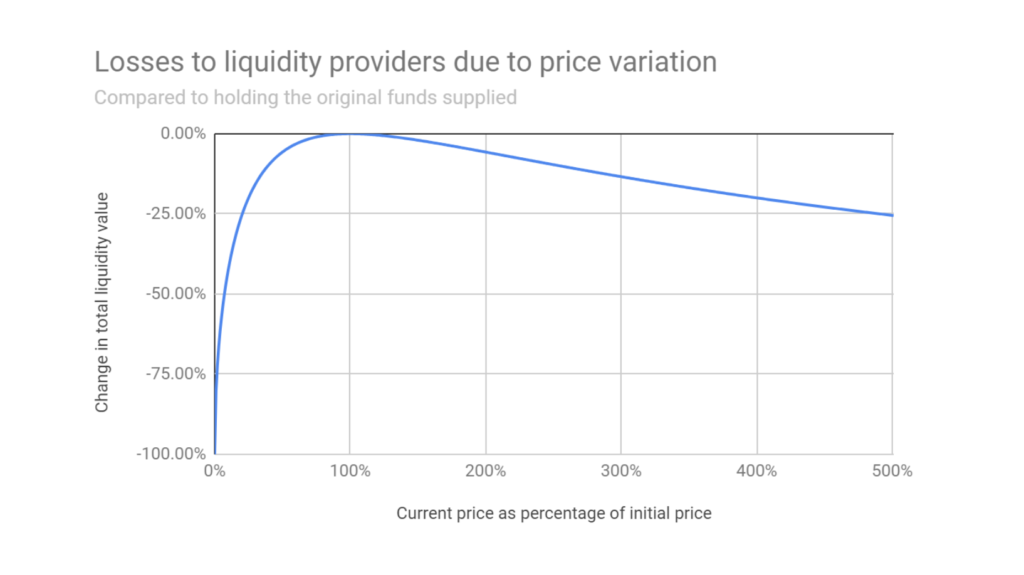
There are multiple specific measures of IL, however the potentially dramatic effect is well demonstrated and visualized in Dinenis & Duijnstee (2023).

Loesch et al. (2021) use definitions of IL they term minimal IL (incurred within the selected trading range) and actual IL (including out-of-range periods). They find that the overall IL in Uniswap V3 often surpasses the fees earned by LPs, meaning that in many cases, LPs would have been better off holding their assets rather than providing liquidity. This is corroborated by Milionis et al., who illustrate how LPs systematically lose money relative to a rebalancing strategy due to price slippage (Milionis et al., 2024).

Loesch et al. find that, for the analyzed pools, the total fees earned since inception were $199.3 million, while the total IL suffered was $260.1 million. This resulted in a net loss of $60.8 million for LPs, indicating that about half of the liquidity providers would have been better off simply holding their assets.

As seen in Figure 1, as the price of the asset deviates from its initial value, the total liquidity value decreases, indicating losses for liquidity providers. The curve shows that even when the asset appreciates significantly, the liquidity value remains below what it would have been if the assets were simply held, highlighting the persistent nature of impermanent loss.

Loesch et al. segment LPs based on the duration of their positions and find that longer-term LPs did slightly better than short-term LPs but still generally suffered from IL. Flash LPs (those providing liquidity for a single block to capture fees from upcoming trades) were the only group consistently making profits, as they did not incur significant IL. This aligns with findings by Milionis et al., who suggest that LPs' performance is heavily influenced by the frequency and magnitude of trades, with those who can quickly adjust their positions being more likely to avoid losses. This can be extrapolated to LPs in AMMs behaving more like LPs in CeFi exchanges, where there is an algorithm external to the AMM entering or exiting pools positions.

Loss vs Rebalancing

Milionis et al. emphasize that LPs face significant losses due to adverse selection, which they quantify as loss-versus-rebalancing, providing a similar perspective on aggregate LP losses to IL. In the context of AMMs, the concept of LVR captures the adverse selection costs incurred by liquidity providers due to arbitrageurs exploiting stale prices. This is different from impermanent loss in that the loss is not incurred purely from the mechanics of price change, but rather from the LP accepting trades at stale or inefficient prices as the pool trends toward the market equilibrium price. It is potentially obvious how a dynamic fee model, if the predictions are good, can mitigate these losses and align fees with market volatility effectively, providing a more sustainable and profitable environment for liquidity providers (Milionis et al., 2024).

The Case for an Adaptive Dynamic Fee System

Dynamic fees are a powerful mechanism in automated market making, offering significant advantages over static fee structures. Milionis et al. propose that by using a model to forecast volatility and adjust fees dynamically, AMMs can mitigate these periods of unprofitability. Their research indicates that aligning fees with market volatility could significantly offset the losses due to IL, providing a more sustainable solution for LPs and takers.

Because impermanent loss is primarily driven by price movements rather than fee levels, our focus is on generating more net fees accrued for LPs based on expected volatility-related measures. This paper does not explore controlling or offsetting impermanent loss itself, but by concentrating on fee generation, we aim to create a more resilient and profitable environment for liquidity providers in decentralized finance ecosystems. This approach ensures that LPs are compensated for their risk exposure during volatile periods by adjusting fees dynamically, thereby enhancing LP profitability and making liquidity provision more attractive.

A note on Volatility and Volume

It could be argued that even if we were able to predict volatility and preemptively increase fees that, ceteris paribus, one might see a decrease in volume as a result of increased fees. However, the implications of this argument becomes less problematic if the volume already increases with volatility.

We find realized volatility and trading volume empirically correlated for both centralized and decentralized exchanges. This supports the idea that dynamic fee systems for AMMs could effectively increase liquidity provider profitability during times of elevated impermanent loss risk by setting higher fees. Conducting a causality test using spot ETH/USDT data from Binance we test if volume Granger-causes volatility and volatility Granger-causes volume using a lag length of 4 with 1-hour time periods for the analysis.

Results in Table 1 show that both hypotheses can be rejected, indicating that there is bidirectional Granger causality between trading volume and volatility. This implies that not only can trading volume be used to predict future volatility, but volatility can also be used to predict future trading volume.

Null Hypothesis	F-Statistic	p-Value	Conclusion
Volume does not Granger-cause Volatility	776.965038	0.000	Reject the null hypothesis
Volatility does not Granger-cause Volume	25.394523	0.000	Reject the null hypothesis

Model-Driven Approach to Dynamic Fees

Higher fees during volatile markets disincentivize arbitrageurs from making money by arbitraging against LP liquidity. It also compensates LPs for the elevated risk they take by providing liquidity. Conversely, lower fees during calm markets incentivize users to trade in the pool. This dynamic adjustment reduces net impermanent loss since when volatility is high, with higher IL and LVR risks, LPs are compensated.

By adjusting fees according to market volatility, the model compensates LPs for increased risk during volatile periods, thereby enhancing their profitability and the attractiveness of liquidity provision in DeFi ecosystems. This dynamic approach addresses the limitations of static fees, offering a more robust solution to mitigate IL.

Why Use Machine Learning for Dynamic Fee Calculation?

• Forward-Looking Predictions: Machine learning models can be predictive rather than reactive. They forecast future volatility, allowing the fee structure to adapt proactively rather than responding to past market conditions. This forward-looking capability can lead to more effective fee adjustments (Milionis et al., 2024).

• Precision and Flexibility: These models are highly flexible and precise in pricing fees. They can capture complex market dynamics and adjust fees with a level of granularity that simple formulas cannot match. This precision ensures that fees are always aligned with the current risk environment, optimizing LP profitability.

• Ease of Model Updates: Machine learning models can be swapped in and out easily instead of being hard-coded into the contract. This modularity is beneficial as market regimes change, allowing for continuous improvement of the fee model without requiring a complete overhaul of the system (Milionis et al., 2024).

• Customization for Different Token Pairs: Different token pairs can have different volatility profiles and risk characteristics. Machine learning models allow for tailored fee structures for each token pair, enhancing the overall efficiency and profitability of the AMM. For instance, highly volatile pairs can have more responsive fee adjustments compared to stable pairs.

• Predictive Volatility Over Realized Volatility: Predicted volatility often provides a better basis for setting fees than realized volatility because it anticipates future market conditions rather than assuming the latest state is the future state. This approach helps in better managing LP risks and ensuring more stable returns.

In centralized exchanges, market makers frequently adjust spreads based on market volatility. During periods of high volatility, spreads are widened to compensate for increased risk and potential price fluctuations. Conversely, during stable periods, spreads are narrowed to encourage trading activity. This dynamic spread adjustment helps manage risk and optimize profitability, mirroring the benefits seen with dynamic fee systems in DeFi.

By leveraging these advanced models, the dynamic fee system not only enhances LP profitability but also improves the overall resilience and attractiveness of the DeFi ecosystem, providing a more sustainable and adaptive trading environment.

Dynamic Fee Model using Risk Prediction

Risk Prediction Model

The risk prediction model used for this paper is a linear model, for which we used Lasso to optimize feature selection and then retrain without regularization after selecting features. Note that in addition to the linear model model we tested a GARCH volatility prediction model, which had somewhat similar (though slightly worse) results, as well as a multi-layer ANN which produced nearly the same predictive power as the linear model. We chose to proceed with the linear model for ease and efficiency of implementation along with satisfactory performance.

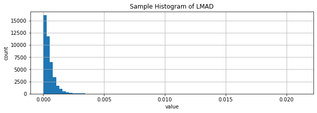
Target and features: Our target and features are variations of log maximum absolute difference (LMAD) for some period. Log-return, $\log (p_t) - \log (p_{t-1})$, is commonly used in price series because inverted returns are comparable in value, for example gaining 100% (doubling value) then losing 50% (halving value) will result in the original price value, but returns of 50% and 100% do not compare well, however $\log$ return of a 100% gain is 0.301 and $\log$ return of a 50% loss is -0.301. For small returns, log return is very close to return. We compare high and low, however the principle remains the same. We define log-absolute maximum difference: $\log ( high ) - \log ( low )$. As with log return and return, in most cases where $high$ and $low$ are relatively near in value, LMAD is approximately $\frac{high}{low}-1$, which is the maximum absolute value of return within the window. There are numerous other specifications using $high$ and $low$ that would produce extremely highly correlated values, for which we would expect nearly the same results. The general concept is that short term price swings, whether the price then reverts or not, can have dramatic negative impact on the LP's potential gains, thus we attempt to capture potential maximal price swings in the immediate future in terms of a target, which seems to be fairly well predicted by related variables in the recent history of series.

We find that LMAD has an extremely right-skewed distribution, and so we use LLMAD $=log(\text{LMAD})$ for preference of well behaved distribution that is much closer to Gaussian, which is well documented to produce better results in linear models. We also use some maximum and mean measures of LLMAD over certain windows. Note that this extreme right skew also presents itself in rolling standard deviation as well, in fact we find that 1 minute LMAD has over 0.9 correlation to the corresponding rolling 1 minute standard deviation of 1-second observations, meaning that LMAD over a longer scale is exceptionally good at capturing volatility information usually requiring higher frequency data to calculate.

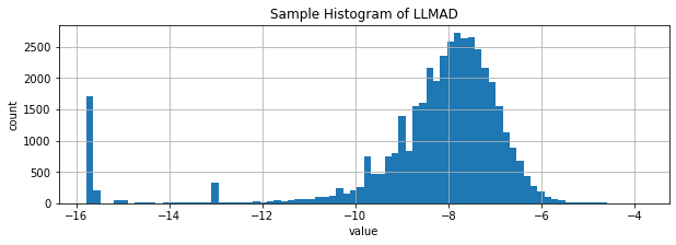
Defining LLMAD and our variations more explicitly:

• $\text{LMAD}_{k,t} = \log(\max_{i} \{ p_i \}_{t-k \leq i < t}) - \log(\min_{i} \{ p_i \}_{t-k \leq i < t})$ where $k$ is a specified time window, for example 1 minute or 5 minutes (in this paper we use $k \in \boldsymbol{N}$ as $k$ minutes)

• $\text{LLMAD}_{k,t} = \begin{cases} \log ( \text{LMAD}_{k,t} ), \ \text{LMAD}_{k,t} > 0\\ \nu, \ \ \ \ \ \ \ \ \ \ \ \ \ \ \ \ \ \ \text{LMAD}_{k,t} = 0 \ ( \nu \ \text{is generally either -9 or -13)} \end{cases}$

• $\text{LLMAD}_{k,t}^{max \ j} = \max_{i} \left\{ LLMAD_{k,i} \right\}_{t-j \leq i < t}$

• $\text{LLMAD}_{k,t}^{mean \ j} = \frac{1}{j} \sum_{i=t-j}^{t-1} LLMAD_{k,i}$

Our target is $\text{LLMAD}_{1,t}$ i.e. future maximal price differences

The initial features we actually select from via Lasso are the following

• $\big\{ \text{LLMAD}_{k,t-1} \big\}_{k \in \{ 1, 5, 10, 20, 40, 80, 160, 320, 640, 1280\}}$

• $\big\{ \text{LLMAD}_{1,t-1}^{max \ j} \big\}_{j \in \{ 5, 10, 20, 40, 80, 160, 320, 640, 1280\}}$

• $\big\{ \text{LLMAD}_{1,t-1}^{mean \ j} \big\}_{j \in \{ 5, 10, 20, 40, 80, 160, 320, 640, 1280\}}$

The choice of values 5, 10, 20, etc. minutes began with the choice of 5 minutes, and doubling each successive number for two main reasons. First, for linear calculations like mean, $n^{-1} \sum_{i=1}^n x_i = \left( \frac{1}{2}(n/2)^{-1} \sum_{i=1}^{n/2} x_i \right) + \left( \frac{1}{2}(n/2)^{-1} \sum_{i=n/2}^n x_i \right)$, which means a linear regression with feature set $\left[ \text{LLMAD}_{1,t-1}^{mean \ 5},\text{LLMAD}_{1,t-1}^{mean \ 10} \right]$ will produce the same target results as variables $\left[ \text{LLMAD}_{1,t-1}^{mean \ 5}, \text{LLMAD}_{1,t-6}^{mean \ 5} \right]$, thus allowing us to treat the 5, 10 as two lags for 5 minute mean, 10, 20 as two lags for 10 minute mean, etc. Nonlinear variables may not analytically turn out as nicely, however for max, $\text{LLMAD}_{1,t-1}^{max \ 5} \leq \text{LLMAD}_{1,t-1}^{max \ 10}$ and $\text{LLMAD}_{5,t-1} \leq \text{LLMAD}_{10,t-1}$.

The second reason is that the dynamics may be apparent over shorter or longer time periods depending on reactivity or noise, and doubling each successive timeframe allows us to analyze and compare substantially shorter and longer timeframes directly against each other.

Data: Our full training set includes data covering 1 Oct 2022 - 31 Dec 2022, which immediately precedes the simulation period in attempt to make the simulation as realistic as possible. The training set is derived from 1-second-frequency Binance exchange "k-lines". We calculate the features described above for each 1-second observation. This is somewhat nontraditional, typically in econometric models the data is sampled at the timescale of the target, however the main justification for that traditional sampling is for purposes of t-scores and other statistics with theoretical requirements of observational noncorrelation. By sampling at 1-second frequency despite the target timescale of 1 minute we are effectively performing the same sort of task as bootstrapping, resampling, or training on synthetic data by increasing the size of the data, however oversampled data is real, nonduplicate data extracted from the true distribution rather than an attempt to recreate the distribution.

For feature selection, the full training set is split 50/50 without randomization, the models are trained on the first set and validated on the second set. It is notable that we tested feature selections for various time windows and months with relatively consistent results especially in selected features, suggesting that this model may perform well treated as time invariant. Consistent performance seen in the dynamic fee simulation further supports the argument for time invariance.

Method for feature selection and coefficient estimation: Using Lasso we choose from a set of penalty parameters ($\lambda$s) by determining which (standardized) feature's coefficients $\beta$ meet the condition $| \beta |>0$ for the given $\lambda$, then rerun using those non-zero features in a standard linear regression, and finally checking correlation between the linear regression's predictions on the test set and the test set's actual values. As will become clear in the Dynamic Fees section's description of the use of z-score to determine fees, it is less important that the average actual and predicted values are near (as might be measured using RMSE) but rather that the ordering and general distribution shape is more correct, hence use of correlation. The choice of features for a pair is determined by the correlation associated with the $\lambda$ for a set of features, however there is some level of arbitrary choice, for example if correlation is only very slightly lower but the number of features is dramatically reduced then the fewer features were chosen in favor of slight performance increase. The OLS regression model with selected features is the model referenced as the risk prediction model. Exact features chosen for each pair can be found in the Appendix.

Dynamic Fees

Building on the insights from the model's performance, we propose a dynamic fee system that leverages the predicted risk from the linear model to set trading fees that reflect current market conditions. The core concept is to offset the potential impermanent loss that LPs may face during periods of high volatility by charging higher fees, while conversely attracting more trading activity during low volatility by reducing fees.

Steps

• Store Predicted LLMAD: Use the predicted value output from the linear model Store this in an array of LLMADs for a specific trading pair

• Calculate Statistical Metrics: Compute the Z-score using of each new predicted LLMAD using $\mu$ and $\sigma$ of prior LLMAD predictions

• Determine Fees Based on Z-Score: If $z \leq -2$, set the fee to the minimum of 18 bps If $z \geq 2$, set the fee to the maximum of 42 bps For other z-scores, use a linear scaling formula: $\text{Fee} = (30 + 6z) \text{ bps}$ This choice is to relatively align with the 30bps Uniswap fee for these pools

• Update Fees Periodically: Let $k$ be the maximum number of blocks needed to calculate any feature of the model For the first $k$ blocks after initialization, use the base fee of 30 bps After 5 blocks, calculate the fee using the method above Repeat this process and update the fee every 5 Ethereum block updates ($\approx$ 1 minute)

Choice of 5 Blocks for Fee Updates: The choice of updating fees every 5 Ethereum blocks, approximately one minute, is based on a balance between responsiveness to market changes and stability in fee structures. Non-algorithmic traders or those with high latency trading systems may not be able to execute a trade within a single block $\approx$ 12 seconds, and so could be subject to unknown and potentially very different fees in the case that the trade is executed with some amount of latency. However, a long interval of a few minutes or more would reduce the system's sensitivity to rapid market changes, potentially increasing LP exposure to volatility without appropriate fee adjustments. It may also provide a more predictable fee structure for traders, though at the cost of adaptability.

The 5-block interval strikes a balance, allowing for timely adjustments to fee structures while avoiding the pitfalls of overly frequent updates. Additionally this choice is informed by common industry practice in high-frequency trading and DeFi market dynamics where minute-level updates are often employed for capturing intraday trends without overreacting to short-term noise.

Results

Historical Fee Collection

The historical fee collection (Figures 2-7 and Table 2) illustrate the cumulative fee over time for different models in WETH/USDT and WBTC/USDC pools on Uniswap V3. The graph compares the standard base fee of 30 bps, the dynamically adjusted fee based on predicted LLMAD from the model, and a normalized version of the dynamic fee. Normalization rescales mean fees from the dynamic model to match the base (30 bps). In this analysis, the cumulative fees collected are calculated each block, and WETH and WBTC are converted back to their corresponding stablecoin using the price for that block to provide a consistent comparison.

The dynamic fee model shows a higher cumulative fee collection compared to the Base Fee model, indicating the dynamic fee system's effectiveness in adjusting to market conditions and increasing profitability for liquidity providers. The higher fee generation by the dynamic model is attributed to its ability to increase fees during periods of high volatility, capturing more revenue when trading activity is riskier or more volatile. This analysis suggests that the dynamic fee system using a dynamic model effectively captures more fees compared to the static base fee, thereby enhancing liquidity provider profitability.

Fee Model	Fees Collected (stablecoin)	Value over Base (%)
WETH/USDT Base (static fee)	11,579,900	-
Dynamic fee WETH	13,766,084	18.8%
WBTC/USDC Base (static fee)	5,721,284	-
Dynamic fee WBTC	6,802,740	18.9%

Historical fee rates applied during the simulation for dynamic models are seen in Figures 4, 5. The fluctuations demonstrate the model's responsiveness to changing market conditions, ensuring higher fees during volatile periods to offset potential impermanent loss and lower fees during stable periods to encourage trading activity. The dynamic adjustment of fees based on market conditions helps maintain a balanced trading environment and protects liquidity providers by compensating them for the higher risks associated with volatility.

Markouts

A very common metric in traditional market making is markouts. The concept behind a markout is that following a trade the price may change, and if the price changes in an adverse direction consistently, i.e. if the LP buys and the price goes down or the LP sells and the price goes up. Usually markouts are a cumulative negative value, suggesting that the LP could have priced more optimally, but it is often nearly impossible for an LP to price absolutely optimally consistently, in which case less negative is preferable to more negative. The principle of measuring markouts is somewhat related to IL, however markouts are better related to LVR in that markouts are generally in a average per-trade basis rather than total portfolio which means the price maybe move up and down in a mean reverting fashion which would having minimal impermanent loss but bad markouts, and bad LVR. Additionally, being on a per-trade basis, the timeframe of a markout is usually much shorter than IL, where markout periods are immediately following the trade, which may be measured in often minutes or seconds.

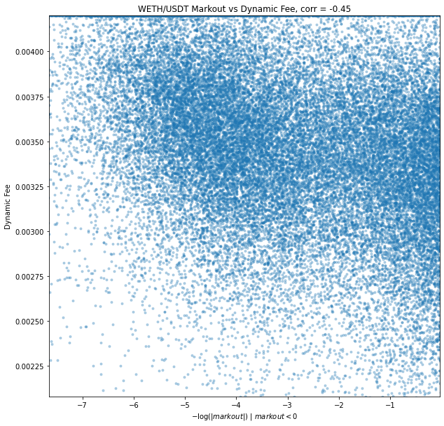
In the the case of AMMs we simulate for this paper, it would be preferable for higher dynamic fees to compensate for bad markouts, which would imply a negative relationship between markouts and fees.

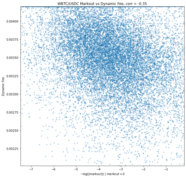
We have calculated and aggregated 2 minute markouts over the simulation. Results demonstrate a significant opportunity cost for LPs. Many markouts are zero or positive, however the markouts of greatest interest are those that are negative because those constitute a direct opportunity loss. Markouts have as strongly left skewed distribution, and so in similar fashion we can use $\log$ to adjust the distribution for a better visual and better understanding of correlation. Since the numbers of interest are negative, we take all negative markouts, take absolute value (to make positive), take the log, and negate again: $- \log (|\text{markout}|) \ | \ \text{markout} < 0$. This is in essence a mirror about the y axis as if the values of interest were positive, and because $\log$ is strictly increasing we can validly use this measure as an order-maintaining variable. We find correlation $\rho=-0.35$ between the dynamic fee and $- \log (|\text{markout}|) \ | \ \text{markout} < 0$, a significant inverse relationship between markouts < 0 and fees as preferred.

Fee Model Evaluation

One of the primary advantages of the dynamic fee model is its ability to dynamically adjust the fee structure according to current market conditions. This ensures that fees reflect prevailing volatility, maintaining a balanced trading environment. By increasing fees during periods of high volatility, the model helps manage risk for liquidity providers, compensating them for the higher uncertainty they face. Furthermore, the use of a linear scaling formula based on z-scores ensures that fees are proportionate to volatility, making the system fairer for all participants. This proportionality promotes a sense of equity among traders and liquidity providers alike. Additionally, the model's reliance on z-scores and a simple linear scaling formula keeps the calculation straightforward, reducing computational overhead and implementation complexity. This simplicity aids in the efficient execution of fee adjustments without imposing significant technical burdens.

However, despite its advantages, the dynamic fee model also presents certain challenges. Implementing the dynamic model and integrating it with the fee structure necessitates more advanced technology and expertise compared to a static fee model. This requirement can potentially increase development and maintenance costs, as specialized knowledge and resources are needed to ensure proper functioning. Moreover, the variability in fees can result in unpredictability for traders, who may prefer stable and predictable fee structures. This unpredictability can be somewhat mitigated by updating fees every five blocks, helping to smooth out sudden changes. Nevertheless, it remains a concern for traders seeking consistency. Additionally, during periods of high volatility, traders may incur significantly higher fees, which could discourage trading activity and reduce liquidity, however on a CeFi exchange spread and slippage can take the place of fees, reducing the comparative cost for the taker. Although this approach prioritizes the protection of liquidity providers by ensuring they are compensated for the increased risk during volatile times, it may inadvertently impact overall market participation.

Future Work

Extension to Other Pairs

The method of feature selection generalizes easily to other pairs or price series of interest. One minute (5 block) update remains seemingly reasonable for any given pair given the argument in this paper, and the choice time periods of features from 1 minute to nearly a full day allow a great deal of flexibility for the predictive dynamics of volatility and price range to be optimally chosen using the given method. The methodology employed to both WETH and WBTC in this paper is the same, but results in differing features (and coefficients), with desirable results in both cases.

Supposing an argument for a more frequent update in volatility prediction, or a slower update (perhaps for a pool that trades infrequently), the target time period could easily be changed. Again, the flexibility of feature selection using training data allows for different features and dynamics for differing target time periods (which is to be expected).

Model Sophistication

As was noted previously, the model, feature set, and fee calculations presented here are all quite simple. A richer set of features for the model, including other measures in addition to or in place of LLMAD as well as variables derived from other time series, for example using data from the WBTC/USDC series to represent systemic risk within a model for WETH/USDT, could provide value. Changing the target itself is completely reasonable. We chose LLMAD due to its desirable characteristics, however other targets could be suitable as well. Further, a more sophisticated algorithm could produce an optimal fee directly rather than require a post-processing step.

The predictive model itself could be extended to nonlinear and n-tensor models (for example GAM, variations of ANN, XGBoost, forest models, etc.) that could find and account for conditional dependence on features. OpenGradient will continue investigating risk modeling in general, and exploration in this area is likely to provide insights into better models for short term predictions that could be used in dynamic fees as well as medium and long term models to be applied to other investing/trading problems.

Fee Model

The fee structure could be modified in many ways. Parameters used for this paper including minimum and maximum fees and scaling could easily be adjusted and optimized. By allowing the base fee, minimum fee, and maximum fee to be adjustable parameters for each pool, the model can better reflect the unique characteristics of each pool. Alternative functions of predictions (as opposed to linear z-score) could be used, or even an ML/AI model tuning the fee structure for optimization, as well as online learning. Additionally, fees could be directional, in CeFi/TradFi market making it is common to only widen the bid or ask side, which is analogous in AMM to increasing the fee for only buy or sell trades.

Furthermore, comprehensive testing across diverse liquidity pools is crucial to ensure the fee model performs well under different pool characteristics. Thorough testing in various pool scenarios can verify the model's robustness and adaptability, ensuring consistent performance regardless of specific conditions.

Conclusion

Well-functioning liquidity provision is necessary for a well-functioning market. Other literature has documented significant frictions and costs for liquidity providers in DeFi Automated Market Makers (AMMs). In this paper, we introduce a potential liquidity efficiency driver in a dynamic fee system for AMMs based on volatility/risk estimation using a simple ML model. By leveraging historical data and volatility dynamics, our model allows trading fees to dynamically adjust in response to market conditions, aiming to offset impermanent loss for liquidity providers and improve efficiency in the market for liquidity. Historical simulations demonstrate that the dynamic fee system consistently generated higher fees compared to a static fee structure, enhancing the profitability of liquidity providers.

The proposed dynamic fee system offers a significant advancement for AMMs by addressing the static nature of trading fees. This approach improves the sustainability and attractiveness of providing liquidity in decentralized finance ecosystems. Incorporating user feedback mechanisms can further optimize the fee model, ensuring it remains responsive to the needs and behaviors of participants. By allowing for dynamic fees, both liquidity providers and those accessing liquidity in the pools can benefit, driving a more efficient and attractive trading venue.

Bibliography

Avellaneda, M. & Stoikov, S. (2008). "High-frequency trading in a limit order book." Quantitative Finance 8, no. 3, 217-224.

Dinenis,G. & Duijnstee, E. (2023). "A Guide through Impermanent Loss on Uniswap V2 and Uniswap V3." Medium, https://medium.com/@compasslabs/the-investor-guide-through-impermanent-loss-on-uniswap-v2-and-uniswap-v3-2b7818999e59

Loesch, S., Hindman, N., Welch, N., & Richardson, M. B. (2021). Impermanent Loss in Uniswap v3. Retrieved from https://arxiv.org/abs/2111.09192.

Elton, E. J., & Gruber, M. J. (2014). Modern Portfolio Theory and Investment Analysis (9th ed.). Hoboken, NJ: John Wiley & Sons.

Campbell, J. Y., Lo, A. W., & MacKinlay, A. C. (1997). The Econometrics of Financial Markets. Princeton, NJ: Princeton University Press (Princeton University Press) (Internet Archive) (Massachusetts Institute of Technology) (Biblio).

Granger, C. W. J. (1969). "Investigating Causal Relations by Econometric Models and Cross-spectral Methods." Econometrica, 37(3), 424-438 (Cambridge University Press & Assessment) (JETI Uni Freiburg) (IDEAS RePEc).

Milionis, J., Moallemi, C. C., Roughgarden, T., & Zhang, A. L. (2024). "Automated Market Making and Loss-Versus-Rebalancing."

Appendix

Linear Model Parameters

WETH-USDT

intercept: -0.13809501340914032

coefficients

$\text{LLMAD}_{1,t-1}$: 0.18694033438620533

$\text{LLMAD}_{1,t-1}^{mean \ 5}$: 0.05895953789579901

$\text{LLMAD}_{1,t-1}^{max \ 5}$: 0.06161016386096607

$\text{LLMAD}_{5,t-1}$: 0.1270665176666954

$\text{LLMAD}_{1,t-1}^{mean \ 10}$: 0.06379694753055712

$\text{LLMAD}_{10,t-1}$: 0.0702867081979839

$\text{LLMAD}_{1,t-1}^{mean \ 20}$: 0.09978892616320731

$\text{LLMAD}_{20,t-1}$: 0.08435978048044984

$\text{LLMAD}_{1,t-1}^{mean \ 40}$: 0.09643320168162073

$\text{LLMAD}_{40,t-1}$: 0.05303044313135884

$\text{LLMAD}_{1,t-1}^{mean \ 80}$: 0.07009809151283451

$\text{LLMAD}_{80,t-1}$: 0.02086389814501841

$\text{LLMAD}_{1,t-1}^{mean \ 320}$: 0.02339777269117423

$\text{LLMAD}_{1,t-1}^{mean \ 1280}$: 0.04844073117207922

else: 0.0

WBTC-USDC

intercept: 0.14275053216323474

coefficients

$\text{LLMAD}_{1,t-1}$: 0.12231823564199638

$\text{LLMAD}_{1,t-1}^{mean \ 5}$: 0.020905377984213384

$\text{LLMAD}_{1,t-1}^{max \ 5}$: 0.06326800868830848

$\text{LLMAD}_{5,t-1}$: 0.18327987170096482

$\text{LLMAD}_{1,t-1}^{mean \ 10}$: 0.08185884246393617

$\text{LLMAD}_{1,t-1}^{max \ 10}$: 0.009224966909740815

$\text{LLMAD}_{10,t-1}$: 0.0826778152449403

$\text{LLMAD}_{1,t-1}^{mean \ 20}$: 0.10436226936878566

$\text{LLMAD}_{20,t-1}$: 0.12156837254695822

$\text{LLMAD}_{1,t-1}^{mean \ 40}$: 0.06714649872050402

$\text{LLMAD}_{40,t-1}$: 0.07666868253855447

$\text{LLMAD}_{1,t-1}^{mean \ 80}$: 0.09402733503137554

$\text{LLMAD}_{80,t-1}$: 0.04229804058740166

$\text{LLMAD}_{1,t-1}^{mean \ 320}$: 0.03716995086288048

$\text{LLMAD}_{1,t-1}^{mean \ 1280}$: 0.0377610199761102

else: 0.0

Alternative model testing

GARCH

GARCH is commonly used for volatility forecasting in financial markets, which made it a natural model to test. The model is specified as follows:

$\sigma_t^2 = \alpha_0 + \sum_{i=1}^q \alpha_i \epsilon_{t-i}^2 + \sum_{j=1}^p \beta_j \sigma_{t-j}^2$

This model is meant to capture the time-varying nature of volatility by considering both short-term and long-term volatility components.

Diagnostic Testing of Model Residuals

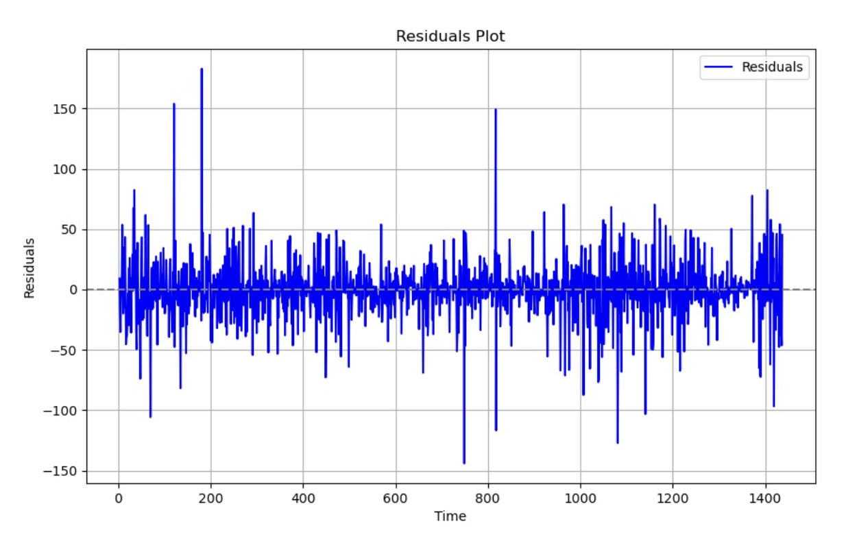
Below is a visual representation of the residuals after fitting the GARCH model onto the data:

Autocorrelation Function (ACF) and Partial Autocorrelation Function (PACF)

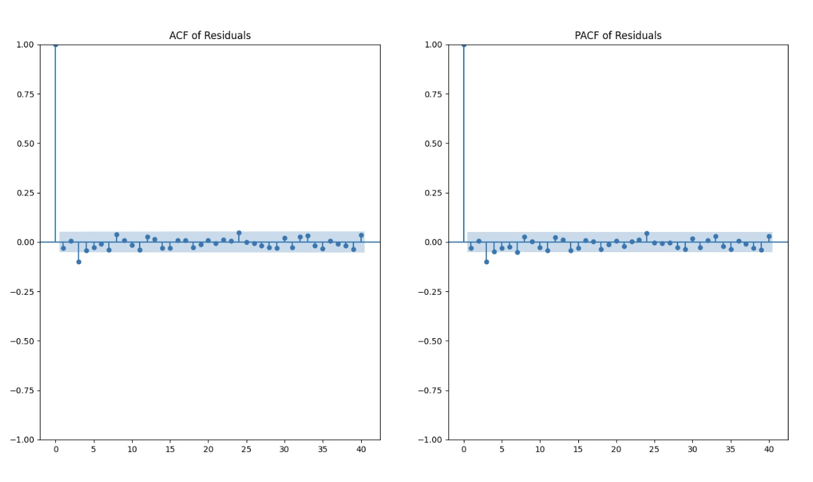
After fitting the GARCH model to the log returns data, we performed more diagnostic tests to evaluate the model's adequacy. Despite the ACF and PACF plots indicating no significant autocorrelation at any time step, the results of these tests suggest the presence of autocorrelation and other patterns in the data that the GARCH model may not fully capture.

Ljung-Box Test The Ljung-Box test assesses whether a time series exhibits significant autocorrelation at multiple lags. The test statistics and p-values for the residuals are shown below:

Lag	Q-statistics	P-value
1	1.244094	0.264684
3	16.385856	0.000945
5	20.167568	0.001162
10	24.678641	0.005989
20	33.116142	0.032764
30	40.298553	0.099210

Variance-Ratio Test The Variance-Ratio test evaluates whether the variance of returns over longer periods is proportional to the variance over shorter periods, thereby testing the random walk hypothesis. The results are as follows:

Lag	Test-statistic	P-value
3	-7.655	0.000
5	-7.417	0.000
10	-6.616	0.000
20	-5.603	0.000
30	-4.948	0.000

ARCH Test The ARCH test examines the presence of autoregressive conditional heteroskedasticity in the residuals. The test statistic and p-values are as follows:

Test-statistic	P-value	Degrees of Freedom	Adjusted R-squared
17.59940734564724	0.06210892802676192	1.7682049731542664	0.06168573286649284

Correlation Analysis The correlation results indicate that our model effectively captures the overall trend in log returns over time. However, it struggles to accurately capture immediate bursts within extremely short timeframes. As shown below, the correlation coefficients increase as the time step duration increases, highlighting the challenge of capturing immediate spikes accurately.

Timesteps	Pearson Correlation
5	0.4987
10	0.5391
25	0.5642
50	0.6653
100	0.7012

ANN

ANN is often a go-to for predictive models. Using the same set of 28 initial inputs as our linear model, namely

• $\big\{ \text{LLMAD}_{k,t-1} \big\}_{k \in \{ 1, 5, 10, 20, 40, 80, 160, 320, 640, 1280\}}$

• $\big\{ \text{LLMAD}_{1,t-1}^{max \ j} \big\}_{j \in \{ 5, 10, 20, 40, 80, 160, 320, 640, 1280\}}$

• $\big\{ \text{LLMAD}_{1,t-1}^{mean \ j} \big\}_{j \in \{ 5, 10, 20, 40, 80, 160, 320, 640, 1280\}}$

which are standardized mean zero, standard devation one, and using an ANN with the following intermediate layers

Dense(128,activation=’tanh’)

Dense(128,activation=’tanh’)

Dense(64,activation=’relu’)

Dense(1,activation=None)

we find results that are essentially indistinguishable from the linear model presented in the paper. It is arguable that a greater diversity of features, other layer specifications, or other variations of ANN could produce different and potentially better results. This is of course part of ongoing research, however these initial results suggest that a linear model specification approximates the relationship between the target and features well, and that even a simple predictive model can provide a great deal of value to the market.

Download the PDF of the paper.

View and run AMM Fee Optimization ETHUSDT and BTCUSDC on the OpenGradient Model Hub.

Gain more insights at OpenGradient Blog.

Follow us on X and join us on Discord.

Developers - Sign up to gain early access to our solutions.